Project 2 Luther

Onto Week 2 and 3! This week we went over web scraping data using BeautifulSoup and Selenium. It proved to be a very important tool in our next project that delt with predicting using Linear Regression. The objective of Project 2 was to build a linear regression model using data we scraped from the web and use the several techniques we learned in class. I was a bit relieved we had two weeks to work on this project so I felt less rushed and more confident I could produce a better work product than my first project.

I quickly knew what topic I would choose. As a UFC fan I decided to predict pay per view buys. I had a couple of ideas of what factors I would be including but in order to fully explore all those features I went over to Tapology (UFC biggest network website) and FightMetric.com to see what type of data would be available.

Luckily FightMetric included a lot of information on one table. Here is what the table looks like below.

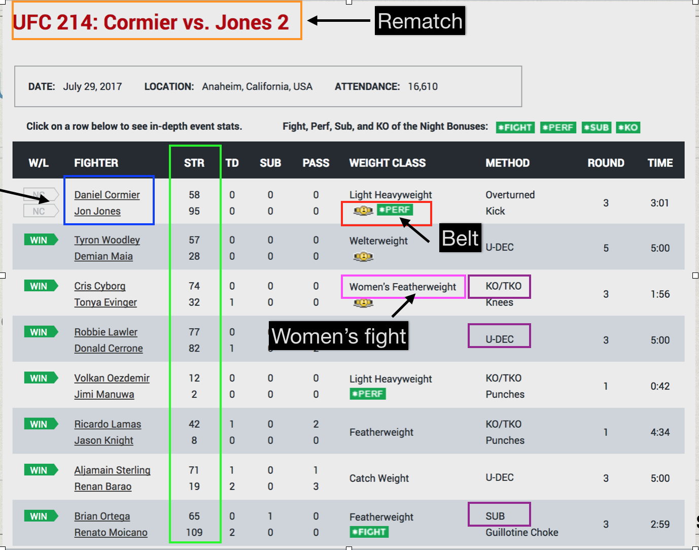
From the table I was able to include the following features: rematch, rivalry, women’s fight, weight classes, fight finishes, title fights, rounds, time on the fights. From tapology.com I was able to collected the number of attendance, ticket revenue, and of course pay per view buys. I decided to create a separate feature called “Fan Favorites” where I included UFC’s top 6 mega stars that have the most fan following and unique star power. This proved to be important as these fan favorites drove a lot of these pay per view numbers.

Exploratory Analysis

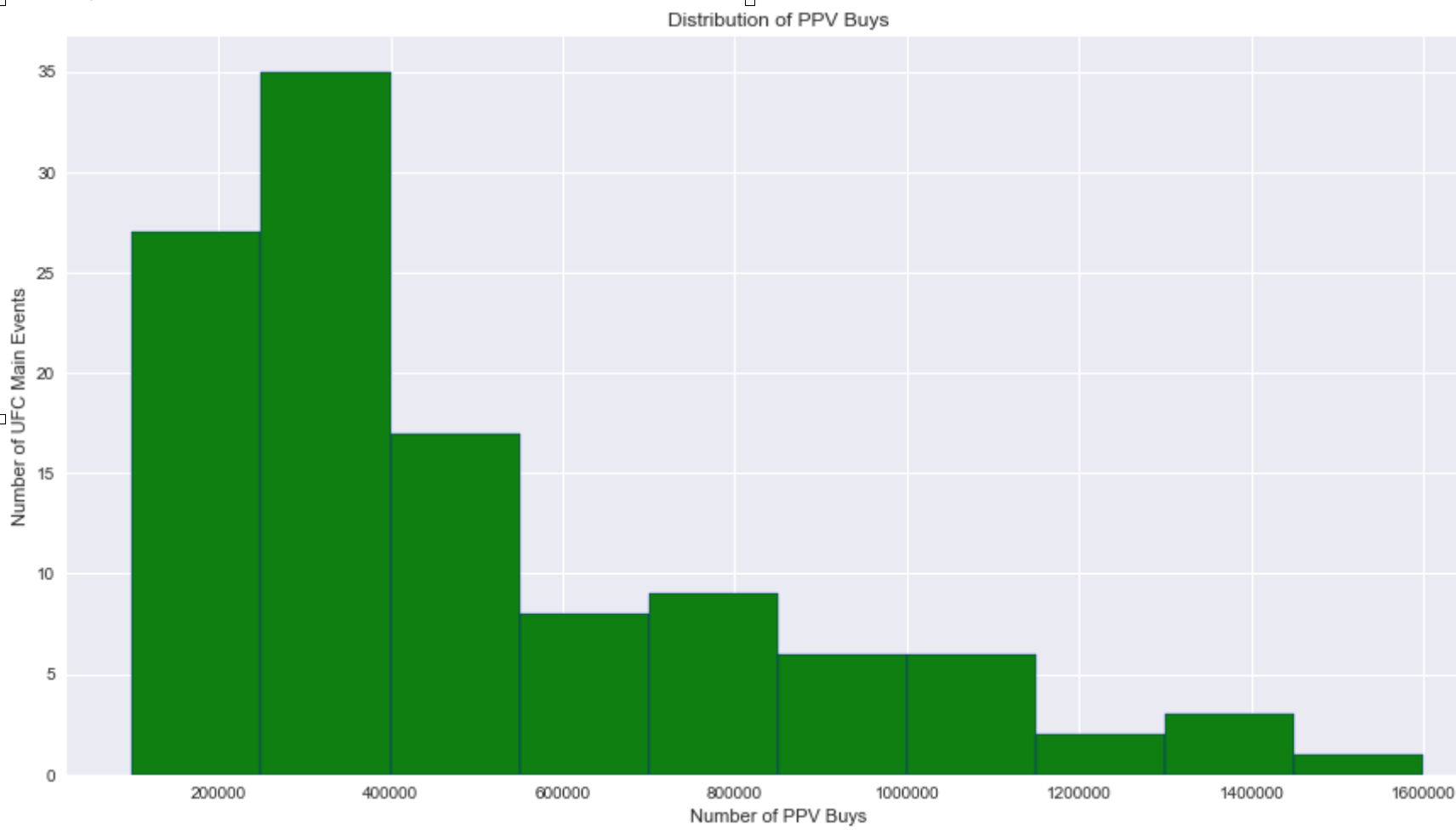
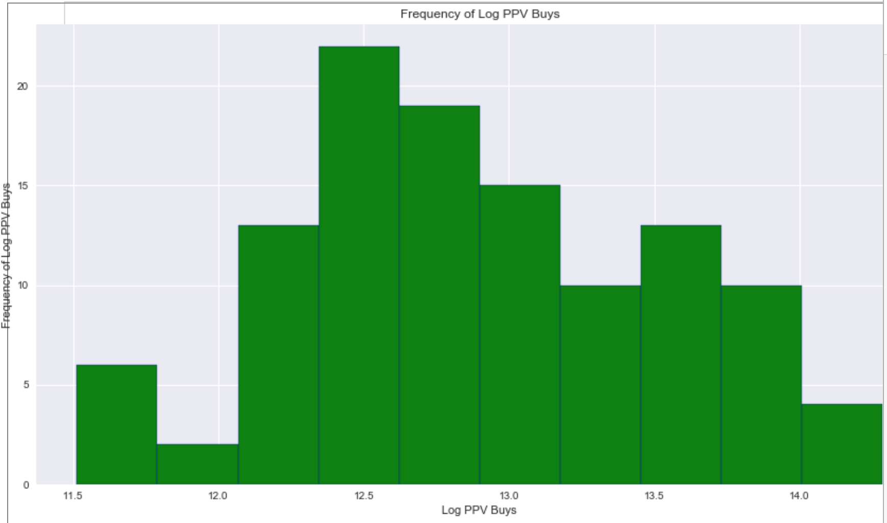
The pay per view horizontal bar graph distribution was positively skewed. In order to make it resemble a normal distribution I had to log transform the target variable. This definitely helped with the skewness and kurtosis of my graph.

Linear Assumptions

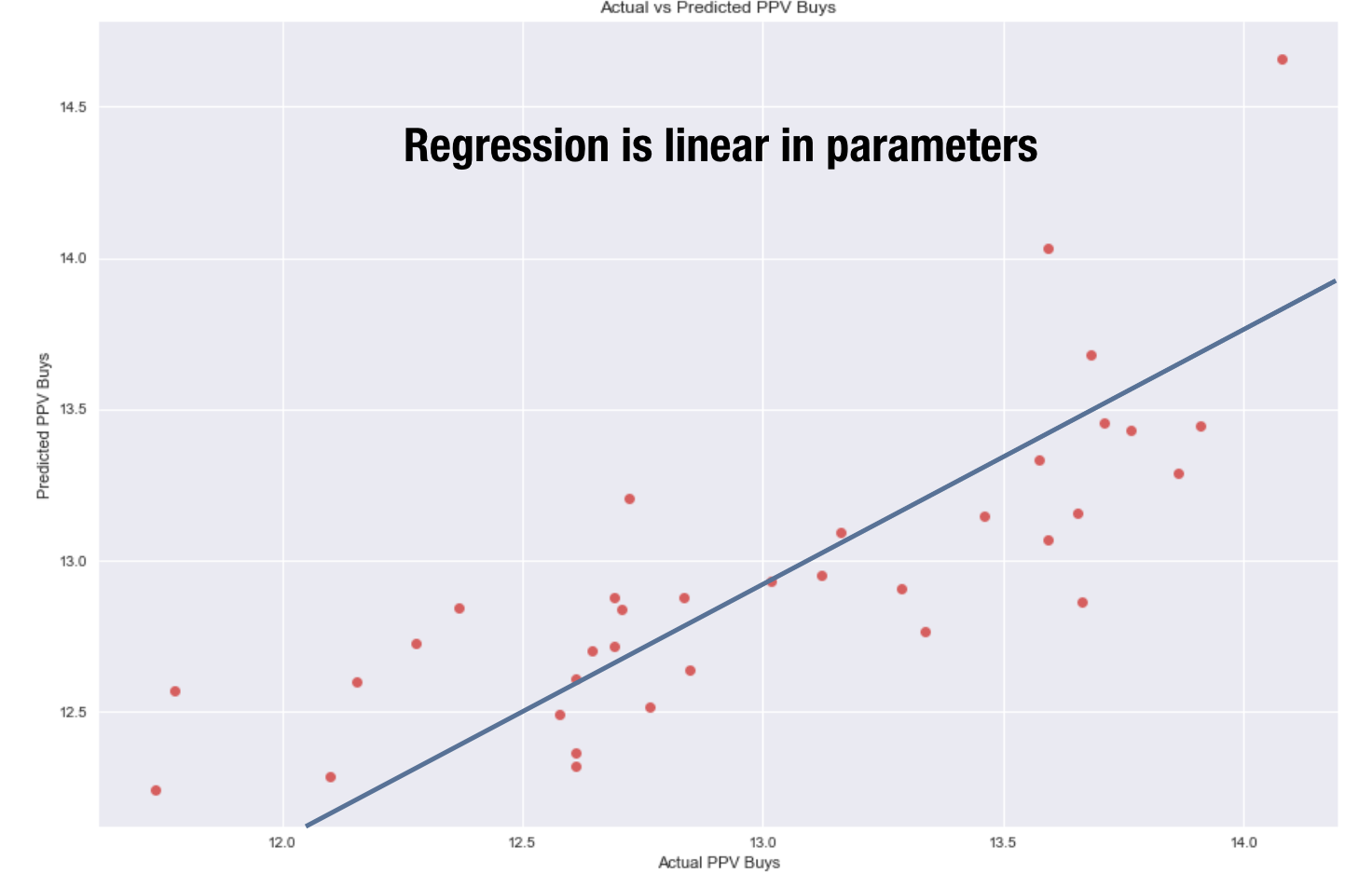
I ensured to check through the linear assumptions of my linear regression model. The first assumption is that the regression is linear in its parameters. In order to inspect this I plotted the actual ppv buys vs predicted. It should symmetrically follow a straight line as you see below.

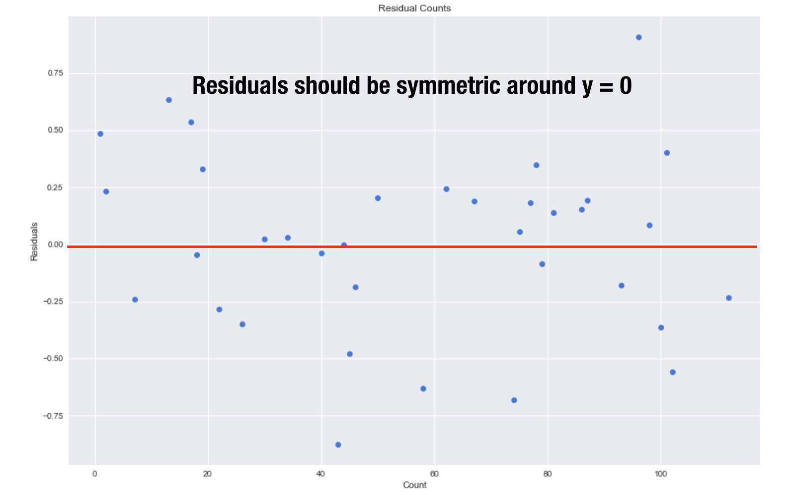
Another thing to check are the residuals. The residuals should be centered around y = 0 and have a constant variance.

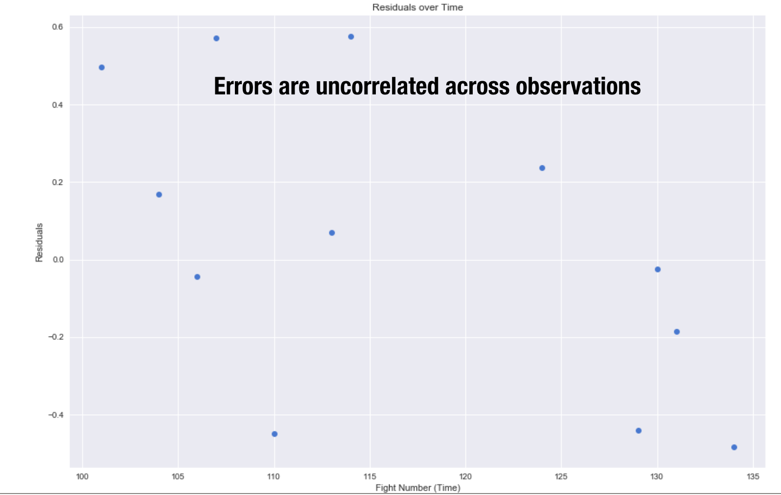
The errors should be uncorrelated so I plotted the residuals against time. As you can see there is no pattern. I also check for multicollinearity which is when two variables are in perfect linear relationship to each other. Fortunately multicollinearity did not exist in my dataset.

Linear Regression Modeling

Train Test Split

Before I began modeling I took a look at the correlations. This is a good starting point to find out which features have the highest impact on your target variable. Fan favorites, ticket revenue, tv rating, rivalries, title fights,and heavyweight fight all had strong positive correlations. On the opposite end of the spectrum, lightweight fights have a negative correlation.

Here is a summary table of my first OLS model. I used statsmodel.formula.api to build this model.

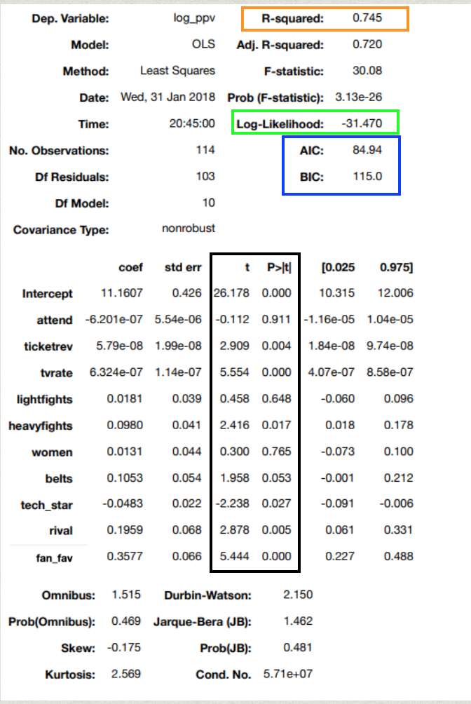
My r2 which is the portion of variation that can be explained by my model is at 75% which is pretty good. During my presentation I went through what every summary statistic translated into my model.

On to checking how my model would perform on out of sample data, I performed a train test split. I designated 30% of my data as my test sample that I did not include in creating my model. This allowed me to test the model against the test sample where I got a r2 of 66%. The r2 went down as aspected because it provides a more realistic representation of how my model will perform in the real world.

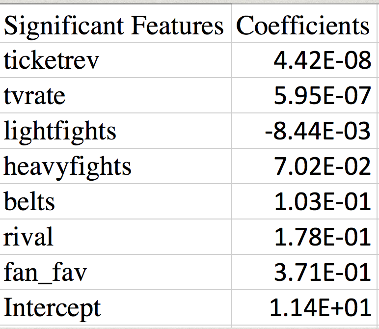
K-Fold Regression

A k-fold regression is essentially performing a train test split multiple times. I performed a 10-fold regression where each fold has an equal chance of being designating as the test set to be tested against. Using this function it identified the significant features by testing the p value. I considered a p value of less than 2% to be considered statistically significant.

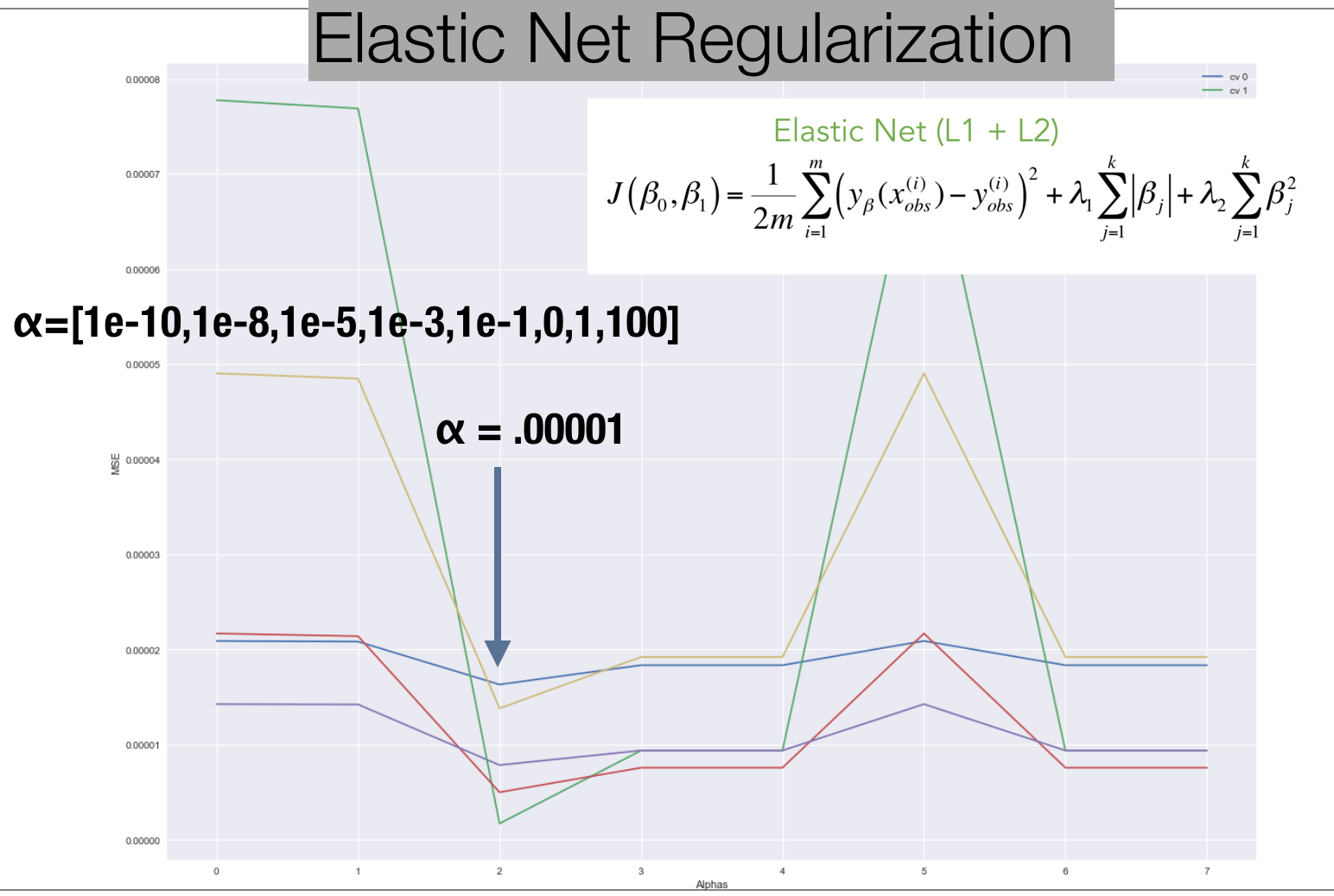
Regularization

In order to avoid overfitting, I used Elastic Net CV to identify the optimal alpha that would correspond with the lowest MSE score. .00001 was the optimal alpha. I set the lasso ratio at .5. However after tweaking the ratio I realized using strictly Lasso produced the highest r2. This is due to Lasso penalizing smaller number less than 1 more. This helped eliminate more features from the model, decreasing the complexity of the model.